Lab 9: SDMs: Model fitting, prediction, evaluation
See also Nan Nourn’s example code with expanded bioclim options for Lab 8 & Lab 9
This lab is a continuation of species distribution models (SDMs)
using the R package, dismo: https://cran.r-project.org/web/packages/dismo/index.html.
The package contains a great vignette and you worked through the first
part of it in Lab 8. You should complete Lab 8’s portion of the vignette
with your species of choice before starting on Lab 9.
For this lab, you will work through Part 2 (Chapters 5-7: Model fitting, prediction, and evaluation) of the dismo vignette. You can find the vignette here: https://rspatial.org/raster/sdm/index.html.
Note that if you want to use a species that does not occur in the dismo vignette bioclim variable range (Mexico, Central & South America), then you need to pull in environmental data from other regions. To do this please see the “Environmental Data” section of the additional code provided in Nan Nourn’s example code with expanded bioclim options for Lab 8 & Lab 9 - this is also linked in Lab 8.
Bioclimatic Variables
In Ch. 4 of the vignette, you were introduced to environmental
predictors, and specifically bioclimatic variables. The dismo vignette
reads in WorldClim bioclimatic
variables. Worldclim interpolates temperature and precipitation from
weather stations to create a modeled representation of these data. Note
that you can create bioclimatic variables from any gridded climate data
source using the command biovars. For example, you could
use satellite remote sensing (direct measures instead of interpolated) -
NASA’s MODIS land
surface temperature and NASA’s GPM
(global precipitation measurement). Or you could use PRISM data if you’re working
in the United States.
The 19 Bioclimatic Variables are listed below. Metadata for these data can be found here.
UNITS: the units for temperature are an order of magnitude larger: °C x 10, and ‘mm’ is the unit for precipitation.
BIO1 = Annual Mean Temperature
BIO2 = Mean Diurnal Range (Mean of monthly (max temp - min temp))
BIO3 = Isothermality (BIO2/BIO7) (×100)
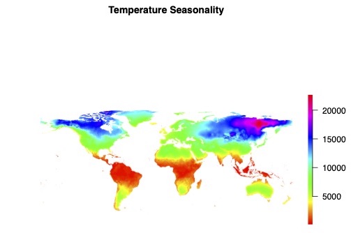
BIO4 = Temperature Seasonality (standard deviation ×100)
BIO5 = Max Temperature of Warmest Month
BIO6 = Min Temperature of Coldest Month
BIO7 = Temperature Annual Range (BIO5-BIO6)
BIO8 = Mean Temperature of Wettest Quarter
BIO9 = Mean Temperature of Driest Quarter
BIO10 = Mean Temperature of Warmest Quarter
BIO11 = Mean Temperature of Coldest Quarter
BIO12 = Annual Precipitation
BIO13 = Precipitation of Wettest Month
BIO14 = Precipitation of Driest Month
BIO15 = Precipitation Seasonality (Coefficient of Variation)
BIO16 = Precipitation of Wettest Quarter
BIO17 = Precipitation of Driest Quarter
BIO18 = Precipitation of Warmest Quarter
BIO19 = Precipitation of Coldest Quarter
What to hand in for Lab 9:
Work through Part 2 (Ch. 5-7: Model fitting, prediction, and evaluation) of the vignette with the example dataset. Choose a different species than the one provided in the vignette (different than the Bradypus species; it would be easiest to select the species you chose in Lab 8 since you already completed that section). Note that the extraction of the environmental predictors occurs in Chapter 4 of the vignette, so if you choose a different species than you used in Lab 8, you will need to go back to earlier portions of the vignette. Re-create Ch. 5-7 of the vignette with your species of interest, constraining the region of your study area to your species known range (ensure that you remove outliers from zoos, incorrect locations by looking up the known range from an independent source).
For more background information on AUC and Spatial Sorting Bias, see the additional text below the QUESTIONS.
NOTE 1: A reminder that if you want to use data from WorldClim outside the dismo vignette data, you should download it; see the “Environmental Data” section of the additional code provided in Nan Nourn’s example code with expanded bioclim options for Lab 8 & Lab 9 - this is also linked in Lab 8.
It is possible that the dismo vignette is using older versions of WorldClim data (version 1.4). These older (but not updated) data can be downloaded directly using getData. The version 1.4 data are outdated so you wouldn’t want to publish anything with them. See above for how to obtain the updated data (2.1). For the lab exercises, it’s ok to use the 1.4 version; you can download 1.4 version data from another area like this:
# Create the folders (directories) "data" and "lab9" - If they exist already, this command won't over-write them.
library(raster)
# Use the getData command
?getData
# World-wide, all bioclim variables, 10 minutes of a degree resolution
w_data_world<-getData('worldclim', var='bio', res=10)
## Warning in getData("worldclim", var = "bio", res = 10): getData will be removed in a future version of raster
## . Please use the geodata package insteadplot(w_data_world)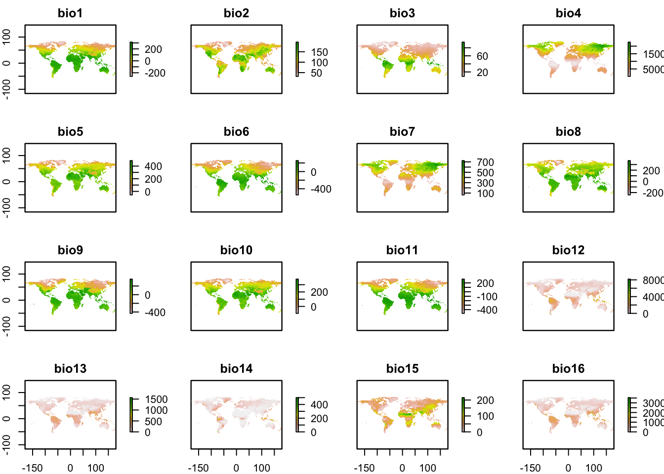
# Region-specific (lon and lat are centered on the area); 0.5 minutes of a degree resolution
w_data_europe<-getData('worldclim', var='bio', res=0.5, lon=5, lat=45)
## Warning in getData("worldclim", var = "bio", res = 0.5, lon = 5, lat = 45): getData will be removed in a future version of raster
## . Please use the geodata package insteadplot(w_data_europe)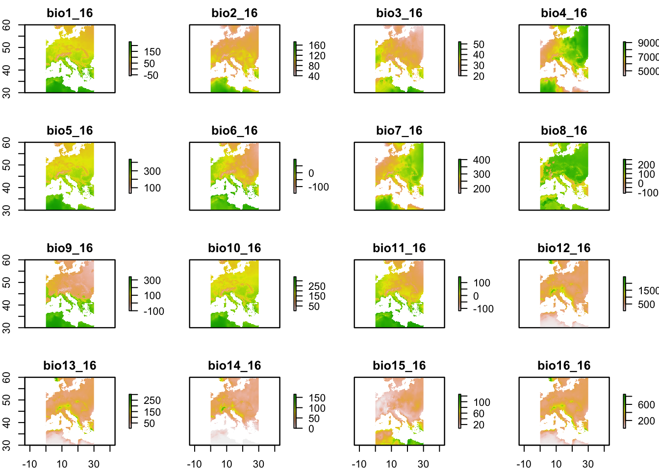
NOTE 2: In Ch. 5-7 of the vignette, when creating the reduced model with a subset of bioclimatic variables (e.g., bio1, bio5, bio12), you can choose to select different bioclimatic variables - see the list of bioclimatic variables above. You should choose a different subset only if the results of your full model (containing the fuller set of bioclimatic variables) suggest a different set, or if you have a priori knowledge of the species-climate relationship.
Show your work (code and output) for this portion of the vignette (Chapters 5-7). You can either add on to Lab 8’s .Rmd file of the vignette that you already produced to create a longer PDF or HTML, or you can hand in a new PDF or HTML with just Lab 9’s section included. Either way, please hand in a PDF or HTML produced from your .Rmd file to show all your work for Ch. 5-7.
After completing the vignette with your species of choice, answer the following QUESTIONS:
QUESTION 1:
Describe the differences you observe in the mapped prediction between the full model, and the reduced model. Which mapped prediction is closer to the known distribution of the species? Provide a source and image (e.g., screenshot) of an independent source showing the range map of the species.
QUESTION 2:
Which model, the full or reduced model, performs better? Why? Include plots and model statistics to help with your explanation.
Extra information on AUC and Spatial Sorting Bias
(SSB): In general AUC improves with larger geographic extents.
As with most of these metrics, you should only compare them across
models that have the same input data (meaning the same records for
occurrences; same number of rows of unique presence and absence
locations). Splitting data into training and testing makes the model
susceptible to being influenced by the actual distances between the
testing and training data in space. To remove this bias, you can subset
the data into training and testing with pairwise distance sampling
(pwdSample in dismo package).
Type the following to see the full details on the
pwdSample command:
library(dismo)
?pwdSample
This
work is licensed under a
Licensed
under CC-BY 4.0 2020, 2022 by Phoebe Zarnetske.