MSU Graduate Spatial Ecology Lab 10
Phoebe Zarnetske: plz@msu.edu; Lala Kounta: kountala@msu.edu; Kelly Kapsar: kapsarke@msu.edu
Last rev. Nov, 2025; created Sep, 2020
Lab 10: SDMs: Modeling Methods
This lab is a continuation of species distribution models (SDMs)
using the R package, dismo: https://cran.r-project.org/web/packages/dismo/index.html.
The package contains a great vignette and you worked through the first
part of it in Lab 8, and the second part in Lab 9. You should complete
Lab 8 & 9’s portion of the vignette with your species of choice
before starting on Lab 10.
For this lab, you will work through Part 3 (Chapters 8-13) of the dismo vignette. You can find the PDF of the vignette here: sdm.pdf, and as HTML here: https://rspatial.org/raster/sdm/index.html.
dismo vignette
.
Types of SDM Models
In Lab 8, you filled in a template describing a particular type of SDM of your choice. See D2L for those summaries as a reference.
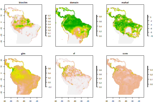
For this Lab, work through Ch. 8-13 (from Modeling Methods through Geographic Modules) with your species’ data from Lab 9. Get as far as you can by building multiple models with different algorithms, and comparing them. Working on the Geographic Models (Ch. 13) is optional.
After completing the vignette with your species of choice, answer the following QUESTIONS:
QUESTION 1:
Describe the differences you observe in the mapped prediction between the different modeling algorithms. Which mapped prediction is closer to the known distribution of the species? Provide a source and image (e.g., screenshot) of an independent source showing the range map of the species.
QUESTION 2:
Of all the models you tried, which model performs best for your species’ data? Why? Include plots and model statistics to help with your explanation. Do you agree that model averaging (i.e., ensemble modeling) is superior to selecting one top model? Why or why not?
 This work is licensed under a
Licensed under CC-BY 4.0 2025 by Phoebe Zarnetske . ```
This work is licensed under a
Licensed under CC-BY 4.0 2025 by Phoebe Zarnetske . ```