Lab 3: Patch Metrics & Spatial Design

RMarkdown version of this Lab

This lab has 2 Parts. Part 1 involves computing patch metrics. Part 2 involves applying patch metrics to design a sampling scheme. You will need to hand in a single PDF produced from your R Markdown file with code, plots, and answers to Questions 1-4, to D2L. When referring to the code below it may be more useful to use the .Rmd file linked above. You will need to be connected to the internet to complete this lab.

At the end of Lab 3 is Homework in preparation for Lab 4 (familiarizing yourself with GitHub).

Part 1: Patch Metrics

We will be using the R package, landscapemetrics to compute patch metrics. Before we can do that, we need to set up the directories and obtain data from the FedData package.

Start working in R:

##### STARTING UP R
# Clear all existing data
rm(list=ls())

# Close graphics devices
graphics.off()

# Set the paths for your work
output_path<-("output")
# if this folder doesn't exist, create it
if(!dir.exists(output_path)){
  dir.create(output_path)
}

# Create the folders (directories) "data" and "lab3" - If they exist already,
#  this command won't over-write them.
data_path<-(file.path("data","lab3"))
if(!dir.exists(data_path)){
  dir.create(data_path,recursive = TRUE)
}

If you previously saved your workspace and want to load it here, do so this way:

load(file.path(output_path,"lab3.RData"))

NOTES on R packages used in this lab:

With R Markdown, it is helpful to install packages locally before knitting (copy this into your R console before you knit).

for (package in c("ggplot2","terra","sf","dplyr")) { if (!require(package, character.only=T, quietly=T)) { install.packages(package) library(package, character.only=T) } }

We can install FedData from CRAN: install.packages("FedData"). Alternatively, We can install the development version from Github, for that we need to install the devtools package:install.packages("devtools") devtools::install_github("ropensci/FedData") library(FedData)
The package landscapemetrics from CRAN: install.packages("landscapemetrics"), or the development version from Github: devtools::install_github("r-spatialecology/landscapemetrics")

Load the packages:

library(dplyr)
library(sf)
library(terra)
library(landscapemetrics)
library(FedData)
library(ggplot2)

The FedData R package is a good way to pull in US environmental data from federal sources. See more here: https://docs.ropensci.org/FedData/. Through FedData we are downloading the 2016 NLCD land cover product for Oregon. We want to work with NLCD data, so it’s important to look up its projection. That can be found in the metadata for 2016 NLCD (navigate to https://www.mrlc.gov/data, scroll down to Data, filter Products Land Cover Time Period 2016. Click on Metadata and search for proj to find the projection information). It’s Albers Conical Equal Area, WGS84. If you need a refresher on Coordinate Reference Systems, refer to this summary sheet (https://www.nceas.ucsb.edu/sites/default/files/2020-04/OverviewCoordinateReferenceSystems.pdf), Lab 2’s links, or resources on D2L.

Practice working with shapefiles and projecting:

# Create a polygon the state of Oregon from the States of US shapefile
if(! file.exists(file.path(data_path,'uss.zip'))){
  download.file("http://www2.census.gov/geo/tiger/GENZ2014/shp/cb_2014_us_state_20m.zip", 
dest=file.path(data_path,"uss.zip"), mode="wb") 
}
unzip (file.path(data_path,"uss.zip"), exdir = data_path)

# Read in the shapefile with rgdal package.
uss <- sf::read_sf(file.path(data_path,"cb_2014_us_state_20m.shp"))

#Take a look at the shapefile info. Its CRS is here: https://epsg.io/42310.
summary(uss)
# What are the first 6 lines of uss?
head(uss)
# Plot it. See that it's showing the states and territories of the US.
plot(uss$geometry)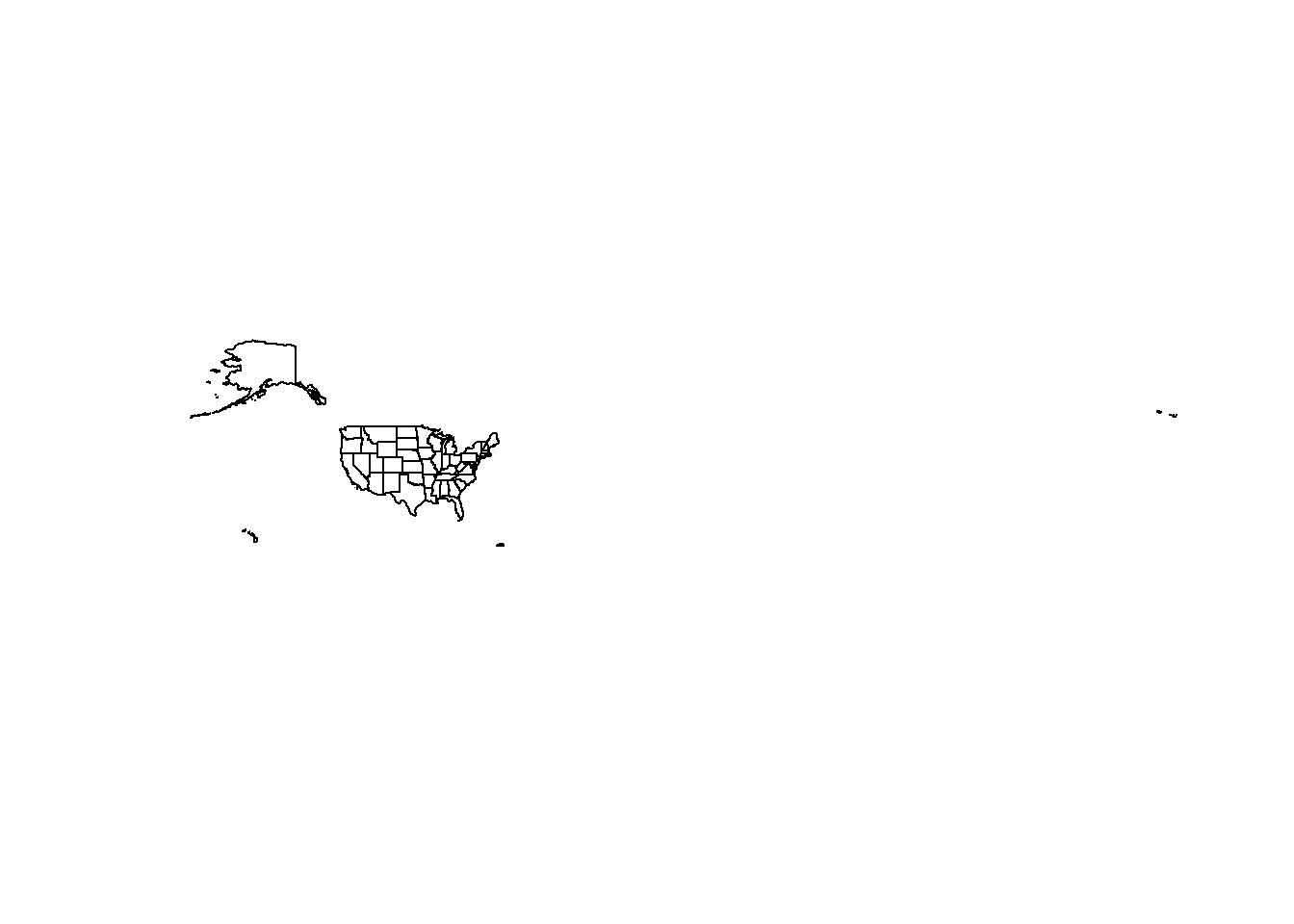

# What are the unique entries in the field, NAME?
unique(uss$NAME)

Projecting We can project these data to match the NLCD data coordinate reference system (Albers, also known as NAD83 / Albers NorthAm). FedData R package returns NLCD data in a different CRS. In general you should avoid projecting rasters because projection of rasters affects their cell values. If you’re working with a raster and a vector in some spatial analysis, project the vector data to match the raster projection.

# Here's the CRS info that FedData returns for NLCD (Pseudo Mercator: https://epsg.io/3857)
merc.proj <- terra::crs("+proj=merc +a=6378137 +b=6378137 +lat_ts=0 +lon_0=0 +x_0=0 +y_0=0 +k=1 +units=m +nadgrids=@null +wktext +no_defs")
# Here's the CRS info for CONUS North America Albers Equal Area Conic (https://epsg.io/5070)
us.aea.proj <- terra::crs("+proj=aea +lat_1=29.5 +lat_2=45.5 +lat_0=23 +lon_0=-96 +x_0=0 +y_0=0 +ellps=GRS80 +datum=NAD83 +units=m +no_defs")

# First let's make a shapefile of just Oregon from the entire US shapefile:
or <- uss[uss$NAME =="Oregon",] 

# Plot Oregon
plot(or$geometry, main="Latitude, Longitude NAD83")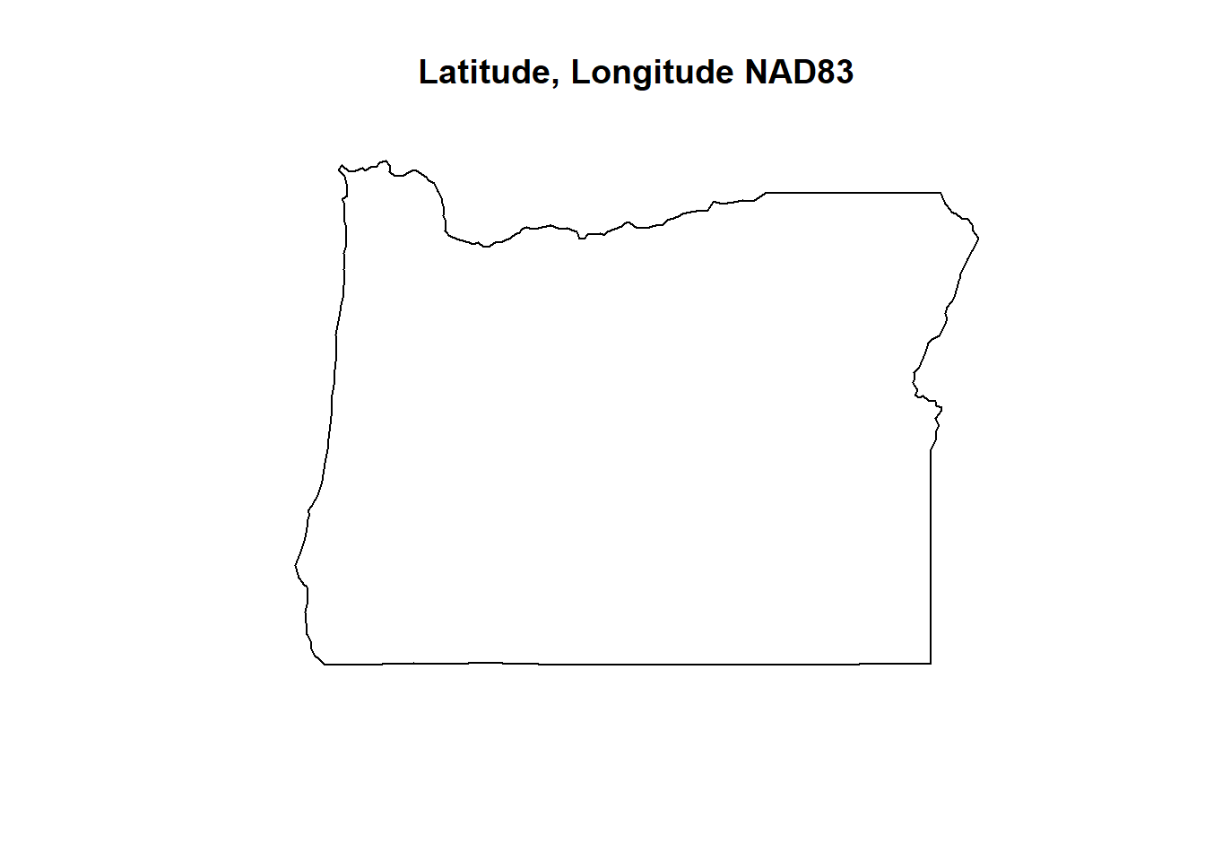

# Practice projecting, and plot again - 
or1<-sf::st_transform(or, us.aea.proj)
plot(or1$geometry, main="Albers Equal Area Conic")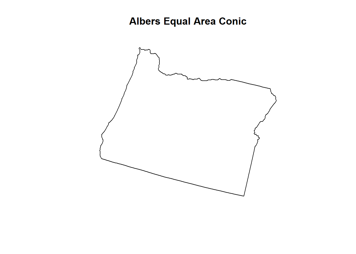

# Supposed you decide to use a rectangle instead of the Oregon polygon boundary.
# Refer to the extent (min and max x and y) of the shapefile, "or1"
summary(or1)
or2 <- FedData::polygon_from_extent(raster::extent(-2294351,-1584307, 2301475, 2899476))
sf::st_crs(or2) <- sf::st_crs(us.aea.proj)
# See how the or2 outlines to the polygon, "or1"
plot(or2)
plot(or1,add=T, col="blue")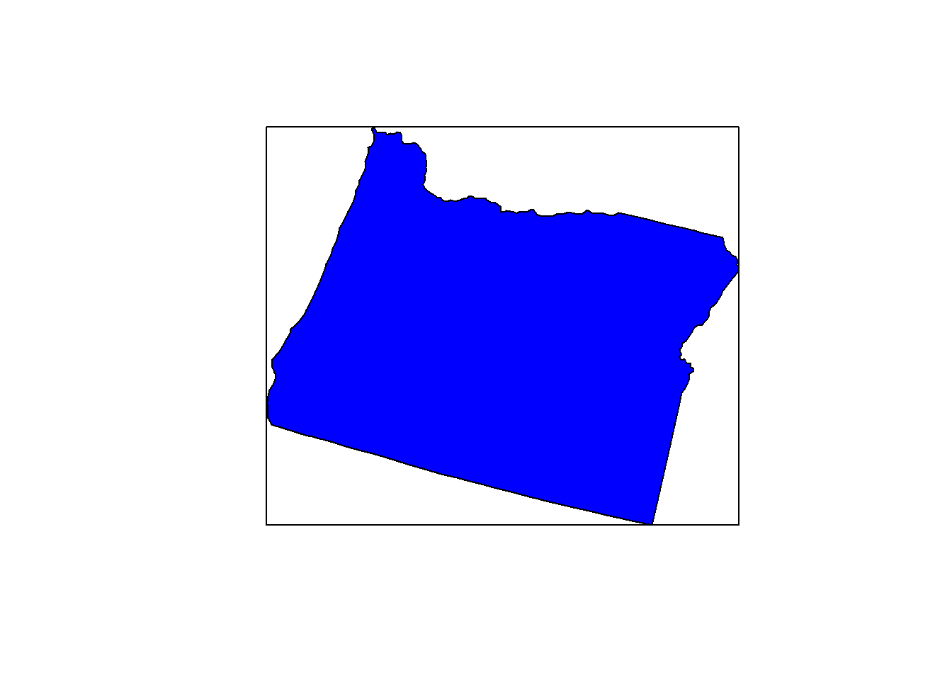

If you wanted to subset out just a portion of Oregon, you could select 1 wildlife management unit. Here is a map of OR Fish & Wildlife Units: https://www.dfw.state.or.us/resources/hunting/big_game/units/bigmap.asp.

Repeat the same process as above, but with the management unit, Hood.

if(! file.exists("mgmt.zip")){
file_name="https://nrimp.dfw.state.or.us/web%20stores/data%20libraries/files/ODFW/ODFW_805_5_wildlife_mgmt_units.zip"
 download.file(file_name,dest=file.path(data_path,"mgmt.zip"), mode="wb") 
}
unzip (file.path(data_path,"mgmt.zip"), exdir = data_path)
mgmt<-sf::read_sf(file.path(data_path,"wmu24poly.shp"))

summary(mgmt) # Its CRS is lcc (Lambert Conformal Conic: https://proj.org/operations/projections/lcc.html)
lcc.proj<-terra::crs("+proj=lcc +lat_0=41.75 +lon_0=-120.5 +lat_1=43 +lat_2=45.5 +x_0=400000 +y_0=0 +datum=NAD83 +units=ft +no_defs")

# Project mgmt to the lcc projection from the Oregon NLCD 2011 (see below)
mgmt1<-sf::st_transform(mgmt, lcc.proj)

head(mgmt1)
unique(mgmt1$UNIT_NAME)
# Select the HOOD Management Unit (where Mount Hood is).
hood <- mgmt1[mgmt$UNIT_NAME =="HOOD",] 
## See where it's located. Plotting and rendering may take a minute because these polygons are complex.
plot(mgmt1$geometry,main="Hood Wildlife Management Unit, Oregon")
plot(hood$geometry,add=T,col="red")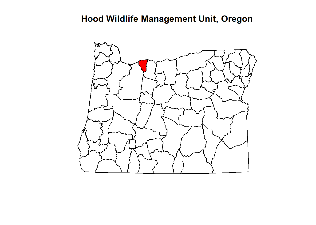

Use the get_nlcd command from FedData to extract the NLCD data for this management unit. FedData does the cropping automatically using a shapefile or raster for “template”. If you run into errors you may need to check what the projection of hood_nlcd is.

?get_nlcd
 
hood_nlcd<-get_nlcd(
  template = hood,
  label="Hood",
  year = 2016,
  dataset = "landcover",
  extraction.dir = paste0(data_path, "/FedData/"),
  )
hood_nlcd # CRS = merc; project hood to overlay them on the same plot.

## class       : SpatRaster 
## dimensions  : 1584, 1220, 1  (nrow, ncol, nlyr)
## resolution  : 30, 30  (x, y)
## extent      : -1999635, -1963035, 2747595, 2795115  (xmin, xmax, ymin, ymax)
## coord. ref. : NAD83 / Conus Albers 
## source      : Hood_NLCD_Land_Cover_2016.tif 
## color table : 1 
## categories  : Class, Color, Description 
## name        :                        Class 
## min value   :                   Open Water 
## max value   : Emergent Herbaceous Wetlands

hood.merc<-sf::st_transform(hood, merc.proj)
# See if you can add a legend - what are the classifications? https://www.mrlc.gov/data/legends/national-land-cover-database-2016-nlcd2016-legend
unique(hood_nlcd)

##                           Class
## 1                    Open Water
## 2            Perennial Ice/Snow
## 3         Developed, Open Space
## 4      Developed, Low Intensity
## 5   Developed, Medium Intensity
## 6      Developed High Intensity
## 7  Barren Land (Rock/Sand/Clay)
## 8              Deciduous Forest
## 9              Evergreen Forest
## 10                 Mixed Forest
## 11                  Shrub/Scrub
## 12         Grassland/Herbaceous
## 13                  Pasture/Hay
## 14             Cultivated Crops
## 15               Woody Wetlands
## 16 Emergent Herbaceous Wetlands

plot(hood_nlcd,legend = FALSE)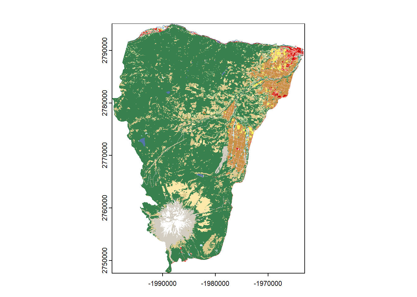
plot(hood.merc,add=TRUE, lwd=2, border='white')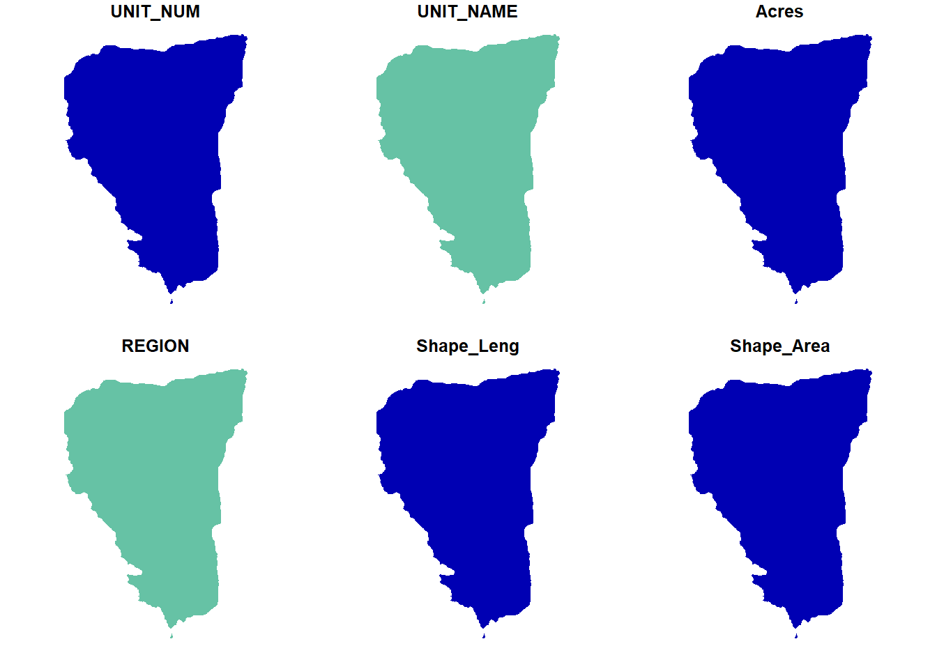

If you have trouble with the FedData package, the code below will import the 2016 Oregon NLCD directly (54 MB); it may take a few mins.

if(! file.exists('or_nlcd.zip')){

download.file("https://ftp.gis.oregon.gov/framework/landuse/NLCD_2016_Land_Cover_OR.zip",

dest=file.path(data_path,"NLCD_2016_Land_Cover_OR.zip"), mode="wb")

}

unzip (file.path(data_path,"NLCD_2016_Land_Cover_OR.zip"), exdir = data_path)

or_nlcd <- rast(file.path(data_path,"NLCD_2016_Land_Cover_OR/NLCD_2016_Land_Cover_OR.img"))

save.image("lab3.RData")

Take a look at or_nlcd from 2011 - it is projected in lcc.

or_nlcd

Crop or_nlcd by hood

hood_nlcd<-crop(or_nlcd, ext(hood))

hood_nlcd <- mask(x = hood_nlcd, mask = hood)

plot(hood_nlcd)

If you want to output a raster as a tif

?writeRaster

writeRaster(raster, "raster.tif")

Now work with the landscapemetrics R package to compute different patch and landscape statistics.

## Check to see if the input data is suitable for computing patch metrics
 
check_landscape(hood_nlcd)

##   layer crs units   class n_classes OK
## 1     1  NA    NA integer        16 ❓

You could proceed to calculate metrics for all different land cover classes (this would take a while). Instead, suppose you are interested in the metrics of “forested” patches in this landscape. First, reclassify into “forest” and “nonforest”. You need to determine what the cover types are:

unique(hood_nlcd)

##                           Class
## 1                    Open Water
## 2            Perennial Ice/Snow
## 3         Developed, Open Space
## 4      Developed, Low Intensity
## 5   Developed, Medium Intensity
## 6      Developed High Intensity
## 7  Barren Land (Rock/Sand/Clay)
## 8              Deciduous Forest
## 9              Evergreen Forest
## 10                 Mixed Forest
## 11                  Shrub/Scrub
## 12         Grassland/Herbaceous
## 13                  Pasture/Hay
## 14             Cultivated Crops
## 15               Woody Wetlands
## 16 Emergent Herbaceous Wetlands

## Look here at the "Class/Value" to figure out which cover type(s) you want: https://www.mrlc.gov/data/legends/national-land-cover-database-2016-nlcd2016-legend. 
#For example, evergreen is 42. However, there are other forest cover types as well. 
# Determine how to make the raster "all forest" not just evergreen. 
hood_for <- hood_nlcd
hood_for[hood_for < 41] <- 0 # make everything below 41 zero
plot(hood_for)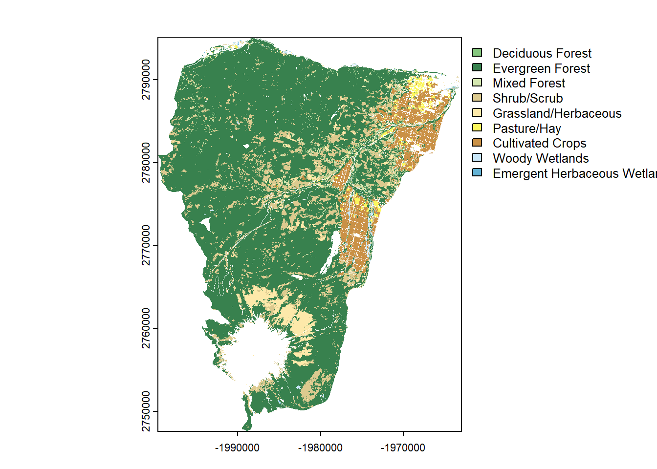

hood_for[hood_for > 43] <- 0 # make everything above 43 zero
plot(hood_for)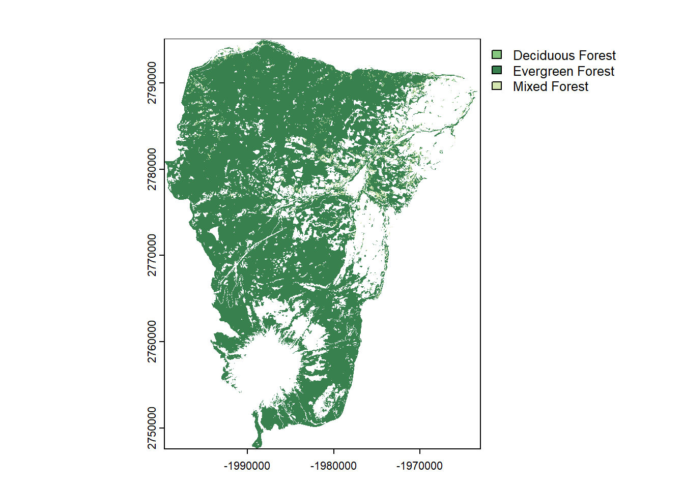

unique(hood_for)

##              Class
## 2 Deciduous Forest
## 3 Evergreen Forest
## 4     Mixed Forest

## Assign 1 value (1) to forest.
hood_for[hood_for == 41 | hood_for == 42 | hood_for == 43] <- 1

The code below follows part of this vignette: https://r-spatialecology.github.io/landscapemetrics/articles/articles/utility.html - check it out for more context and if you would like to try other commands not covered here.

## Check to see if the input data is suitable for computing patch metrics
check_landscape(hood_for)

## Look at the distinct patches for this landscape
show_patches(hood_for)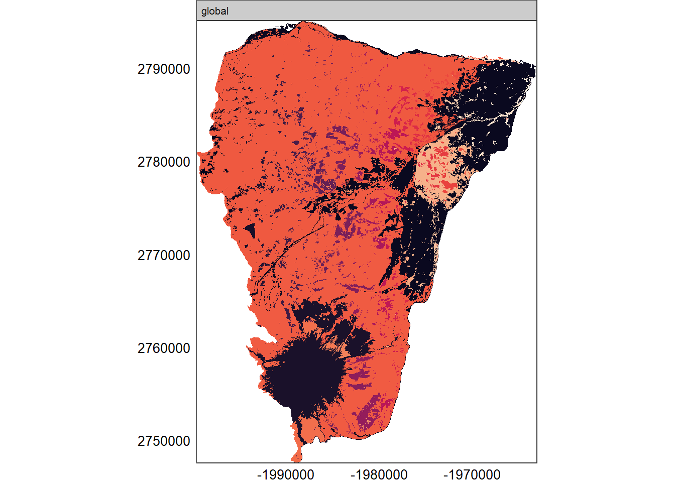

## Show patches of each class (we have 2 classes: 0 for non-forest and 1 for forest)
show_patches(hood_for, class = "all", labels = FALSE)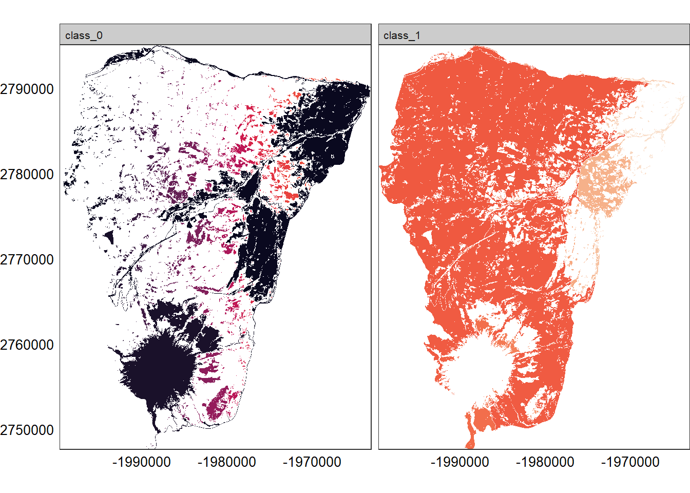

## At the patch level, compute patch metrics
hood_metrics <- calculate_lsm(hood_for, what = "patch")

## Look at the different types of metrics at the patch level. Note that you can compute these metrics at the patch, landscape, or class levels.
list_lsm(level='patch')

#look at just Forested patches; subset out class==1 for forest
hood_metrics_for <- subset(hood_metrics, class == 1)

# Since hood_metrics_for is a tibble, we use this format for plotting (using ggplot2). 
# Note that the y axis scale varies by plot when faceting by metric below. 
# We use a log10 scale for the x axis to visualize the spread more effectively.
hood_for_metrics_hist<-hood_metrics_for %>%
     dplyr::select(value, metric) %>%
     na.omit() %>%
     ggplot(aes(value, fill = metric, color = metric)) +
     geom_density(alpha = 0.2)+
     scale_x_log10()+
     facet_wrap(~metric, scales="free_y")
hood_for_metrics_hist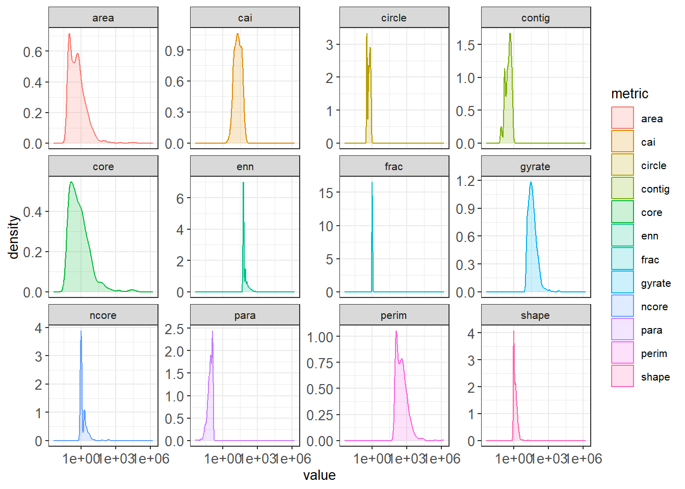

## Determine if any patch metrics for forest are correlated
show_correlation(hood_metrics_for, method = "pearson")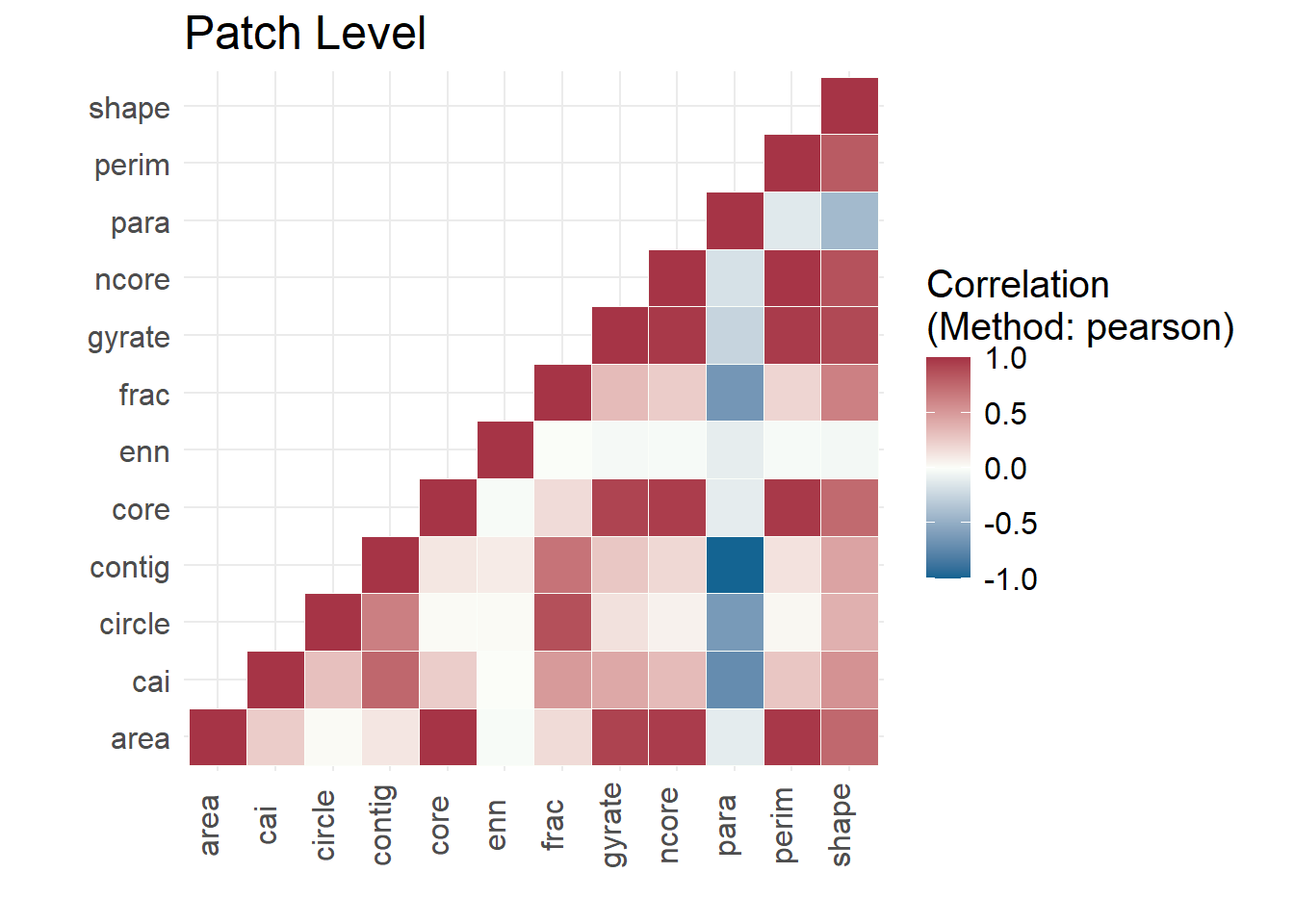

QUESTION 1:

How do the patch metrics from landscapemetrics help you understand how an organism interacts with its environment? For 3 metrics of your choice, explain in 1-2 sentences what the metric tells us about an organism’s interaction with its environment. Feel free to use examples. Refer to the list_lsm() results above. You may also want to refer to the landscapemetrics documentation for more in-depth coverage https://r-spatialecology.github.io/landscapemetrics/articles/general_background.html

QUESTION 2:

Repeat the process above (see Repeat the same process as above, but with the management unit, Hood), but select a different management unit than Hood. Compare your other management unit patch metrics with the ones for Hood Management Area. Briefly, how do the patch metrics for Forested areas and non-Forested areas compare between the two management areas? Optional: make some plots showing the statistical distributions of patch metrics across the two areas (e.g., a histogram of patch area, by class, by management unit).

Part 2: Study Design

You decide to study the interactions between Spotted Owls and Barred Owls in Oregon forests (do a little internet searching to understand why studying these 2 species together is important, and what their habitat requirements are).

QUESTION 3.

Use GBIF data to add to one of the management unit maps you created above. On this map, overlay “recent” point locations of each of these species (as different symbols and/or different colors). Justify the timeframe you chose for the occurrences. Add a descriptive title to the plot. Add a legend, scalebar (with units), and north arrow for your map. You may want to reference Lab 2 and below for some potentially helpful code.

In the terra package see the options for each command: ?plot to plot the raster ?points() to add points for the species ?sbar() to add a scalebar

QUESTION 4.

If you had unlimited resources, describe how you would sample the 2 management units to obtain new occurrence data next year for both species. Are there specific forest attributes that would be helpful to know in addition to just “forest vs. non-forest”? Use terminology from the Lecture and Discussion about sampling.

Homework in preparation for Lab 4:

In Lab 4 we will introduce GitHub, a versioning program helpful for collaborating and tracking changes in code. You can think of it as a Google Docs version for tracking code changes (you can also use it with text). If you are familiar with GitHub, no need to go over the following, but if you are not familiar, please work through the following tutorials [personally, I use the Desktop version but any version will work]:

At a minimum, please complete this first short tutorial ahead of Lab 4: